Constant-acceleration equations connect speed, elapsed time and displacement when acceleration stays constant over the interval. They are useful for a basic calculation or for checking a motion estimate, but they do not describe every real vehicle or machine cycle with one number. This guide keeps the sign convention explicit and shows four independently recomputed examples.
Core equations and examples
Choose a positive direction first. Use the same length and time units throughout, and treat acceleration as signed: a negative value points opposite the positive direction. In the example rows, v0 is initial velocity, v is final velocity, a is constant acceleration, t is elapsed time, and s is displacement from the starting point.
[gs_table id=”10979″]
Know which equation removes an unknown
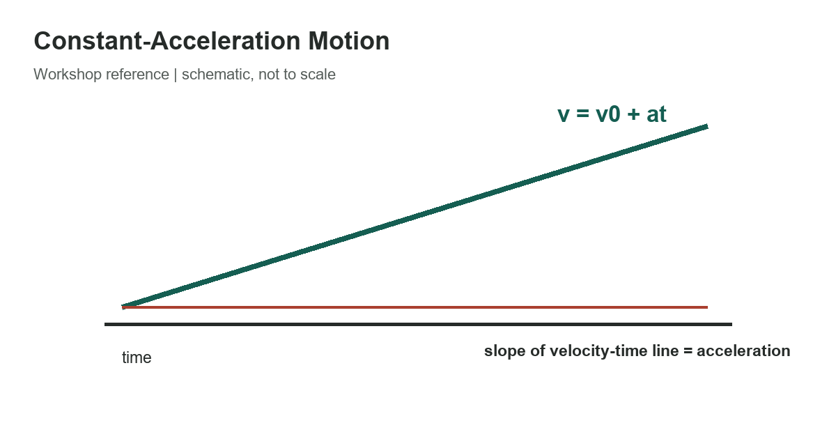
For final velocity when time is known, use v = v0 + at. For displacement over a known time, use s = v0t + one-half at squared. The velocity-displacement relation v squared = v0 squared + 2as is useful when time is not known. With constant acceleration, average velocity over the interval is (v0 + v)/2, so displacement is average velocity multiplied by elapsed time.
These equations are algebraic forms of one-dimensional kinematics, not a substitute for a free-body analysis. They assume acceleration is constant during the chosen interval and ignore effects not represented by the inputs. If acceleration changes substantially, divide the motion into intervals and calculate each one with suitable initial and final conditions, or use a method that models variable acceleration.
Read the signs before calculating
Suppose an object begins at rest and accelerates at 2 m/s squared for 5 seconds. The final velocity is 0 + 2 times 5 = 10 m/s. Its displacement is 0 times 5 + one-half times 2 times 25 = 25 m. The average velocity is 5 m/s, and 5 times 5 seconds also gives 25 m. Agreement between the two methods is a useful arithmetic check.
For a stopping calculation, choose the direction of travel as positive. A deceleration then has a negative sign. If v0 is 20 m/s and a is -4 m/s squared, set final v to zero in v squared = v0 squared + 2as. Solving gives s = (0 – 400) / (-8) = 50 m. The positive displacement is in the original travel direction.
Use consistent units
If speed is in meters per second and time is in seconds, acceleration must be in meters per second squared and displacement will be in meters. Do not insert a speed in miles per hour into an SI equation with seconds without converting it first. Dimensional checking catches common errors: acceleration multiplied by time has units of velocity, while acceleration multiplied by time squared has units of distance.
For a unit conversion, 1 m/s equals 3.6 km/h. Convert an entire set of inputs to a single system before calculating, and round at the end to a precision supported by the measurements. A calculator may return many digits, but that does not make the measured inputs more accurate.
Do not treat the ideal model as a stopping guarantee
Vehicle braking is not usually a single constant-acceleration event from the instant a hazard appears. Driver perception and reaction add distance before braking begins. Tire condition, brake condition, load, grade, surface, weather and speed affect the actual motion. A calculation using a selected deceleration is a model, not a safe following-distance recommendation or road-test substitute.
Likewise, a motor or lift may accelerate, coast, brake and settle through different control phases. Use the equations separately for an interval only when its acceleration approximation is justified. For equipment design, include the manufacturer’s limits, control logic, load, stopping method and applicable safety requirements; do not infer a load capacity from a kinematics equation.
Calculation checklist
Write down the initial conditions, define positive direction, convert units, choose the equation that contains the knowns and desired unknown, and preserve signs through substitution. Check the units and whether the result’s sign and magnitude make physical sense. If a square root appears, interpret the sign using the chosen direction and problem context. State the constant-acceleration assumption beside the result.
When the data are noisy or acceleration varies, a single end-point equation may hide important dynamics. Use time-series measurements or a verified engineering model instead, and document assumptions. For a simple estimate, the equations remain useful because each result can be traced to stated inputs and checked independently.
Related references: exact inch-to-metric length relationships, rose chucking reamer dimensions, and ribbed-neck bolt dimensions. Each covers a separate shop-reference task.
Sources and scope
The equation set and one-dimensional constant-acceleration assumption are presented in OpenStax College Physics 2e and OpenStax University Physics. All numeric examples in the table were recalculated from the displayed equations.